Oct 18, 2026

Introduction

CNS GLBR is a macOS application that takes a GRBL 1.1 laser engraver from idea to finished part: importing a drawing, nesting, G-code, running the job, monitoring it and keeping records. I wrote it for my own machine (a 290 × 170 mm working area and a diode laser of about 10 W optical output), so every feature has been tried on real work, on plywood, rather than just on paper.

The main ideas:

•   Your work is not lost. If the connection drops, the power flickers or you stop a job, you can pick it up again from the same point.
•    Settings can change mid-job. Laser power and travel speed can be adjusted while the job is running or paused, with no need to stop and restart.
•    Everything is visible up front. Time, dimensions, working-area limits and cost are known before you press Start.
•    One tool instead of several. The vector editor, nesting, raster engraving, tracing, queue and log all live in one window.

The rest of this overview goes through every panel: what it is for, how it works and what it gives you in practice.

A note on the interface: the application's interface is available in English and in Russian. It follows the language of your Mac by default and can be switched at any time from the Language / Language menu (the change takes effect after a restart). The screenshots in this overview show the English interface.

The layout of the window

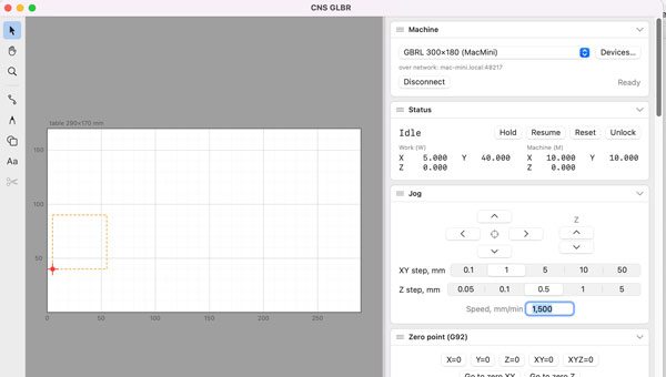
The window has two parts: the canvas ("Work table") on the left and a column of panels on the right. The canvas shows the machine's working area, your drawing, the toolpath of the job and a red marker for the head (where the laser beam is). Everything you control is on the right.

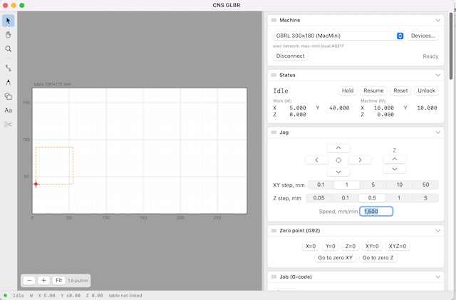
The main window: the work table on the left, the panels on the right.

Panels can be collapsed, dragged and reordered, and the order is remembered between sessions. That way only what you need at the moment is on screen: while setting up, "Jog" and "Zero point"; while running, "Job" and "Status". If new panels don't appear after an update, choose Panels → Reset layout from the menu.

The benefit: a laptop screen doesn't turn into a wall of buttons, and the workspace adapts to the stage you're at.

Machine and Status

Machine is the connection panel. Choose a machine profile, then a port (USB) or a network connection, and press Connect. The "Devices…" button opens the list of machines: each has its own profile with the working area, parameters and bridge address, and you can create your own with whatever values suit you. For a network connection, the panel shows the address and port.

Status shows what the machine itself reports: its state (Idle, Run, Hold, Alarm), machine and work coordinates, current power and speed, and the Hold, Resume, Reset and Unlock buttons.

Why it matters: everything the program does is based on the machine's real state. The movement buttons are disabled until the machine is ready, and an Alarm is shown straight away and cleared with a single Unlock button, with no console commands.

The benefit: machine profiles save you from setting things up again. Switching between machines takes seconds.

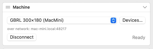
The Machine panel: profile, connection and state.

Manual control

Jog has arrow buttons for X/Y and separate buttons for Z. The XY step is chosen from 0.1 / 1 / 5 / 10 / 50 mm and the Z step from 0.05 / 0.1 / 0.5 / 1 / 5 mm; the speed is set in a field. Two step sizes cover two situations: bringing the head roughly up to the workpiece, and positioning it precisely on an edge.

Zero point (G92) has the buttons X=0, Y=0, Z=0, XY=0 and XYZ=0, which set the zero of the work coordinates wherever the head is now. "Go to zero XY" and "Go to zero Z" send it back. This is the reference point for every job that uses absolute coordinates.

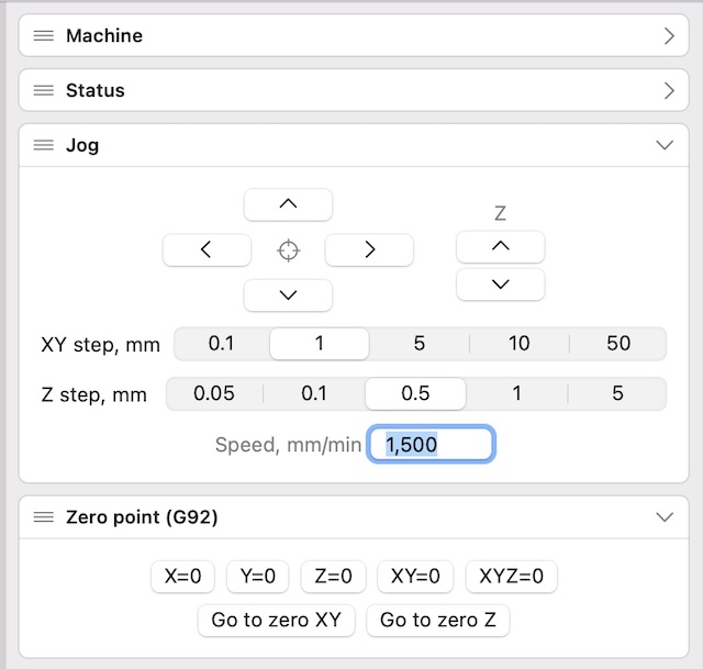
The Jog and Zero point (G92) panels.

Laser test is a button that fires the beam at the chosen power for as long as you hold it. With "Latch" switched on, one press turns the beam on and the next turns it off. There are built-in safeguards: power is capped at 5 %, the beam switches itself off after 30 seconds, and releasing the button turns it off. What it is for: seeing the spot and the focal point, and lining the head up with an outline, without any risk of scorching the material.

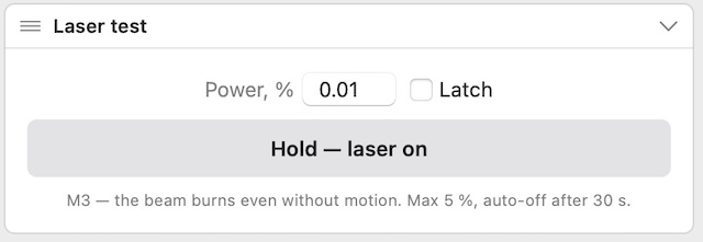
The Laser test panel: power-limited and with an automatic cut-off.

The benefit: all the positioning is done without a live beam at full power.

Table and head

This panel links "where the head is now" with "where it sits on the table". At the top it shows the head's coordinates on the table (and the work coordinates) and the size of the working area.

If the machine doesn't do homing, its machine zero is simply wherever the head was when it was switched on. In that case the program doesn't know where the limits of the working area are. The fix: put the head at a known position (a corner or the centre), choose that position in the "Head is currently at" list and press "Tie table to head". "Reset" removes the link, and it also resets itself when you reconnect.

Why: the bounds check works against the real 290 × 170 mm working area. A job that would go outside it is not started, so the head never runs into the end of its travel part-way through. You can switch the check off with the "Don't check bounds" tick box in the Job panel.

The benefit: even without limit switches or homing, the program still knows the edges of the table, with a single calibration.

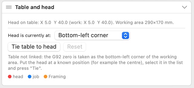
The Table and head panel.

The Job (G-code) panel

This is the heart of the program. "Open…" loads a ready-made G-code file; jobs made from a vector drawing, a raster image or the test matrix arrive here automatically once you press "Create job". After loading, the program analyses the file and shows:

•    the number of lines, the dimensions in mm, and the maximum S (power) and F (feed rate);
•    an estimated time, calculated with a model of the GRBL motion planner that takes acceleration and the machine's actual settings into account (read from its $ settings; without a connection, typical values are used);
•    the coordinate mode (relative to the head's current position, or absolute from the G92 zero);
•    warnings about any problems in the file.

The buttons are Start, Pause / Resume, Stop, Preview… and Back to start. A progress bar shows how far along the job is, and before it starts the program checks that everything fits inside the working area on the table.

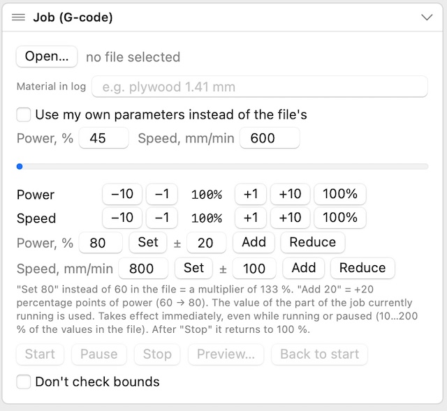
The Job panel, with the power and speed controls that work while a job is running.

The Preview window shows the toolpath and the expected time and can play the job back step by step. It also has the "Start from here" button (see below).

Three more things in this panel:

• "Use my own parameters instead of the file's" lets you set one power (0–100 %) and one speed (1–6000 mm/min) for someone else's file without editing it by hand;
• an estimate line with a correction from the log and the cost (see the log section);
• a "Material in log" field, for example "plywood 1.41 mm".

The benefit: the program tells you how long the job will take, and whether it will fit, before work begins rather than after.

Changing settings while a job is running

This is one of the program's biggest advantages. Under the progress bar in the Job panel there are two sets of controls, for power and for speed. Each works as a multiplier on the values in the file:

•    the −10, −1, +1, +10 and "100%" buttons change the multiplier in steps;
•    "Set" applies an exact value: if the file says 60 % and you want 80 %, the multiplier becomes 133 %;
•    "Add" and "Reduce" work in percentage points: "+20" turns 60 % into 80 %.

Changes take effect immediately, both while the job is running and while it is paused, within a range of 10–200 % of the values in the file. For the part of the job being cut at that moment, it is that part's own value that is used, so layers with different power settings don't get mixed up. After Stop, the multiplier returns to 100 %.

A typical case: an engraving is coming out too faint, so you add power without stopping the machine or losing your position. Or a cut hasn't gone all the way through, so you reduce the speed on the fly until the result is right.

If, after stopping, you need to redo the job from the first point, "Back to start" returns the head to the job's starting point. You then change the parameters and press Start again.

The benefit: you find the right setting by looking at the result on the actual material rather than guessing. Before, a single adjustment meant stopping the job and starting over. Here the workpiece stays put and the job runs without a break.

Resuming after an interruption

Cutting and engraving take a long time, and the workpiece is expensive. In an ordinary program, a dropped USB connection, a frozen computer, a closed laptop lid or an emergency stop means losing the whole job. CNS GLBR handles this properly: an interrupted job can be finished from the point where it broke off.

How it works

•    When a job starts, the program saves a checkpoint to disk: the full G-code, the job's name and the head's starting position.
•    As the job runs, it records how many lines the machine has confirmed as executed (not merely "sent", but actually "accepted", which makes the count more accurate).
•    Even if the program has been closed or the computer restarted, the next time you launch it a "Resume from where it stopped" line appears in the Job panel, with the note "N of M lines done".
•   The "Forget" button deletes the checkpoint if you don't need to finish the job.

What happens when you press it

The head must be where it stopped. The program works out the right line in the job from the head's current position, restores the necessary modes (power, feed rate, offsets) and carries on with the rest. If it can't determine the exact place (the head is not on the toolpath), it doesn't guess; it tells you why.

"Start from here"
The same mechanism is available in the Preview window: pick any point on the toolpath, and the head travels from the start point to it without cutting and continues the job from there. The program asks for confirmation first, and the working-area limits are checked just as for a normal start. Typical uses: skipping a section you have already checked, redoing only the last part, or finishing a contour that wasn't cut all the way through.

The benefits

• No wasted material or time: the workpiece stays on the table and nothing has to be repeated.
• No doubling up: areas that have already been burned are not burned again.
• Before resuming you can adjust power or speed, if the interruption happened because the settings weren't right.
• A resumed job is recorded in the log as a separate run ("… (resumed)"), so the time accounting isn't lost.

Important: resuming relies on the workpiece and table not having moved and the zero point not having been disturbed. After an interruption, don't move the head by hand, and don't press Reset unless you really have to.

Job queue, job log and cost

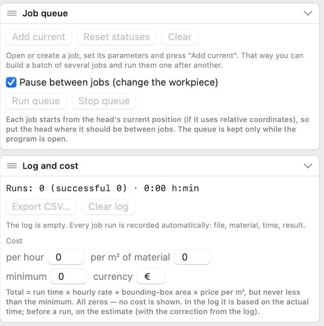
The Job queue and Log and cost panels.

Job queue

A batch of parts means several jobs run one after another. You open or create a job, set its power and speed, and press "Add current". The queue receives the finished G-code with your own parameters already applied, so each job keeps its own settings.

• Each row shows the job's name, dimensions, time and status (waiting, running, done, failed); the order is changed with the arrow buttons.
• The totals show the remaining time and the cost of the whole batch.
• "Pause between jobs": after each job the program waits while you change the workpiece and position the head, and starts the next one only when you press "Next". Without the pause, jobs run back to back with a one-second gap.
• If a job breaks off or you press Stop, the queue stops rather than carrying on regardless.
• "Reset statuses" puts everything back to waiting, so you can run the same batch again.

Limitations: each job starts from the head's current position (for jobs in relative coordinates), and the queue is kept only while the program is open.

Log and cost

Every run is recorded automatically: the file, the material, the date, the actual time against the estimate, the dimensions, the maximum S and F, and the outcome: "Done", "Stopped", "Interrupted", ALARM or "Connection lost". You can add a note to any entry ("came out a bit faint, added +5 %"). The panel shows the last 30 entries; the rest (up to 1,000) are in the log file and in a CSV that opens in Excel and Numbers, with Cyrillic text intact.

The log gives you two useful things:

• A time correction. Once there are at least three successful runs longer than 30 seconds, the program takes the median of actual time against estimate and adds a line to the Job panel: "according to the log, the real time is usually ×…". The estimates get more accurate with every run.
• Cost. The rate is set with three numbers: a price per hour of machine time, a price per square metre of material and a minimum charge per job (the default currency is the euro, and it can be changed). The total is time × hourly rate + the area of the bounding box × the material price, but never less than the minimum. Before a run the cost is based on the estimate; in the log, on the actual time. If all three numbers are zero, no cost is shown.

The benefit: you have data on settings, and for customer orders a real cost price and an accurate expectation of the time, not guesswork.

Framing: tracing the outline

Before you start, it's important to see exactly where the work will land. Framing moves the head around the rectangle of the job's dimensions, so you can see whether the part fits on the workpiece without wasting any material.

• Size: width and height in mm; either "From the head's current position" or an X/Y point.
• Speed and power: a power of 0 means no beam, and the maximum is 10 %, so you can follow the guide dot.
• The outline is checked against the machine's working area, and at the end the head returns to where it started.

Power in Framing is deliberately limited: it is a position check, not a processing step.

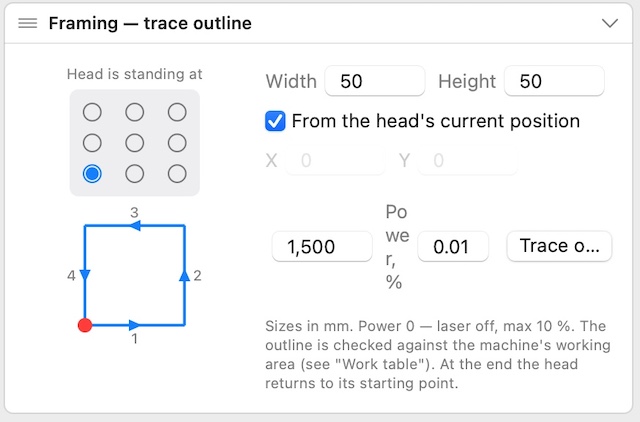
The Framing panel: a position check, not a processing step.

The benefit: a cheap check of "does it fit, and where will it sit" before an expensive operation.

SVG / DXF import and the drawing editor

This is where a drawing becomes a job. "Open SVG/DXF…" loads a file; arcs are converted to Bézier curves on import, so circles stay smooth rather than turning into polygons. If the drawing needs scaling, set the size in the "Scale, %" field; you can also crop to the page boundary (the viewBox).

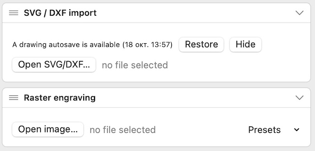
The SVG / DXF import and Raster engraving panels.

Layers and modes

Each colour or layer of the drawing is a separate operation with its own power, speed and number of passes, so engraving, outlining and cutting right through can each be set differently. The program works out the order itself: lower-power operations run before stronger ones, and inner contours before outer ones. That way a cut-out part doesn't fall away before the holes and the pattern have been burned into it.

Node editor and Bézier curves
Paths can be edited directly on the canvas: drag nodes, adjust the tangent handles, and select many nodes at once and move them together. There is also copy and paste, scaling, rotation, joining segments into a single contour, and offsetting a closed contour inwards or outwards, for example to allow for the width of the burn or to make a frame.

If the offset is deeper than half the width of the shape, the program does not produce an inverted contour; it declines, and this is covered by tests.

Groups

A part often consists of dozens of paths: the outline, holes, a pattern. "Group" combines them into one object and "Ungroup" takes them apart again. A group is moved, copied and nested as a whole, and when segments are joined, contours from different groups are not merged. Copies get their own groups.

Nesting on a sheet

The sheet size, margin from the edge, gap between parts and permitted rotation (none, 90° or 45°) are set in the panel; "Nest" then lays the parts out according to their real shape, not as rectangles. A part is its outer closed contour together with whatever is inside it, and a group counts as one part. Thanks to groups, a blank made of 74 paths is laid out as one piece instead of being scattered.

Tracing

A raster picture can be turned into contours, with a threshold, a minimum area, a tolerance and a "light instead of dark" option. The result is an ordinary drawing: you can edit it with nodes, cut it, fill it and nest it.

The benefit: from file to finished job in one window, with no separate editor or converters. The "Create job" button hands the result to the Job panel, where the time and limits are shown.

Raster engraving

A photograph or picture is engraved line by line: the head moves back and forth while the power varies with the brightness. The panel offers three modes:

• Grayscale: smooth tonal transitions; darker areas burn more strongly, lighter ones less;
• Threshold: pure black and white, suited to logos and line drawings;
• Dithering: tones are rendered by the density of dots, as in newspaper printing.

Settings

• Size and position: width in mm (the height follows the proportions) and an X/Y offset from the head's position. If the head is in the bottom-left corner, the offset is the picture's margin from the edges.
• Quality and speed: the spacing between lines (0.02–1 mm) and the feed rate. A finer spacing gives a cleaner result but takes longer.
• Power: a minimum and a maximum in %; the darkest areas never burn harder than the maximum.
• Tone: brightness, contrast, gamma, threshold and invert.
• Direction: "Bidirectional" halves the time; rotating each pass (0°, 45°, 90°) helps to hide banding when you use several passes.
• Frame: the "Cut a frame around the picture" switch adds a cut-through outline after the engraving, with its own margin, power and speed. It is one operation rather than two separate runs, with no risk of the position shifting between them.

A tested setting for 1.41 mm plywood

Operation	Setting
Engraving (threshold)	threshold 40, contrast 20, gamma 1.3, max. power 25 %, 1,000 mm/min, line spacing 0.1 mm, bidirectional
Cut and frame	100 %, 400 mm/min

At this power the cut goes through in roughly one pass; as a rule of thumb, burn-through starts at about 0.3 J per millimetre of travel. The hint in the panel suggests a general starting point (5–40 %, 2,000–3,000 mm/min, 0.1 mm spacing), but only a test on an offcut will show the right setting for your own material.

The benefit: raster and cut are done in a single job without the position shifting, and the tone controls are right there in the panel.

Presets

It would be a shame to lose a setting you worked out on a material. The "Presets" menu is in the raster engraving block and in every vector layer. You save the current settings under a name, with the material and a note, and next time apply them with one click.

• A built-in set is there from the first launch; you can restore any built-in presets you've deleted, and your own are left untouched.
• They are stored in a single file, ~/Library/Application Support/CNSGLBR/presets.json, which you can copy to another computer or keep as a backup.

The benefit: finding the right setting for a new material is done once, and after that it comes from your library.

Test matrix and Console

Test matrix

A way of finding the right setting for a new material in a single run. You set a range of power and speed, the size of each square and the gap between them; the program builds a grid of squares in which the columns vary the speed (from lower to higher, left to right) and the rows vary the power (from bottom to top). The bottom-left corner is where the head is standing.

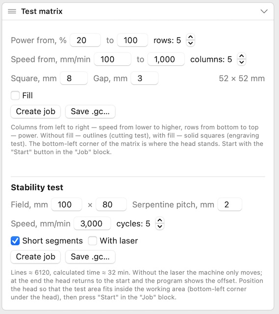
The Test matrix and Stability test panels.

• Without fill: outlines, for testing cutting.
• With fill: solid squares, for testing engraving; the line spacing is set separately.

You can run the result as a job or save it as a .gc file. After the run you can see which square came out best and take its power and speed into a preset.

Console

A log of the exchange with the machine and a line for typing GRBL commands by hand (the "Send" button), plus "Copy all" and "Clear". You won't need it for everyday work, but it helps when setting the machine's parameters ($110, $120, $30 and so on) and when tracking down a fault: everything the machine says is shown exactly as it is, and is easy to forward when asking for help.

The benefit: the matrix replaces days of trial and error with a single run on an offcut.

Network bridge

The machine can sit by one Mac (in my case a Mac mini) while you work at another. The reason is that a laser produces a lot of smoke, and it is better kept in a separate, ventilated room.

On the computer with the bridge installed (the CNSGLBR-Bridge.pkg package), the machine's USB port is made available over the network. The bridge is configured under System Settings → CNS GLBR Bridge: port, password, switching the service on, and a log. In the application you choose a "network" connection with the address and the same password.

Protection is built into the bridge itself:

• Password. Without the right password, no connection is made.
• One client only. If another program is already controlling the machine, a second connection is refused.
• Protection against a dropped connection. If no data arrives from the application for 10 seconds, the bridge closes the connection and, if the option is enabled, stops the machine: a pause, then a soft reset. Motion stops and the laser goes out, so there is no risk of the head being left with the beam on if the laptop freezes.

The benefit: the laptop can be well away from the machine, and a long job doesn't depend on a single USB cable or on unpleasant surprises.

Safety and tested settings

A laser is a dangerous tool, so the program protects you in layers:

• power limits in the manual modes (test 5 %, Framing 10 %) and an automatic switch-off of the test beam after 30 s;
• a working-area check before every start;
• Pause, Stop and Hold/Reset always within reach;
• a watchdog in the bridge for dropped connections;
• autosave of the drawing: if the program closes unexpectedly, it offers to "Restore" it.

Settings tested on 1.41 mm plywood (LT-80W-F45 laser, about 10 W optical output):

What we're doing	Power	Speed
Cutting through	95 %	400 mm/min
Raster (threshold 40, contrast 20, gamma 1.3)	up to 25 %	1000 mm/min
Frame around the picture	90 %	400 mm/min

Rule of thumb: energy per millimetre of travel = power × 60 ÷ speed (mm/min); burn-through on 1.41 mm plywood starts at roughly 0.3 J/mm. The machine is set up with $110 = $111 = 1000 mm/min and $120 = $121 = 30 mm/s².

Always: keep a fire extinguisher close by, switch on the air assist, wear protective glasses, test any new material on an offcut first, and never leave the machine unattended.

Key benefits

1. CNS GLBR is built around making laser work predictable and ensuring nothing is lost when something goes wrong.
2. Resuming after an interruption. A dropped connection, a stop or a closed program doesn't cost you the workpiece: the job is finished from where it broke off, and "Start from here" lets you join the toolpath at any point.
3. Changing settings on the fly. Power and speed can be adjusted while the job runs or is paused, so you tune the setting by the result on the material.
4. Predictability. Time, dimensions, the working-area check and the cost are known before you start, and the log refines the estimate over time.
5. Batches and records. A queue, a log with notes and CSV export, and rates for machine time and material.
6. The whole route from drawing to part. SVG/DXF, nodes and Béziers, groups, shape-based nesting, raster and tracing in one program.
7. Network and reliability. A password-protected bridge that stops the machine if the connection is lost.
8. Your own settings. Presets and the test matrix make finding the right parameters for a new material quick.

Installation and requirements

The program runs on macOS 12 and later. To install it, drag CNSGLBR.app into Applications; to connect to the machine over the network, also install CNSGLBR-Bridge.pkg on the computer the machine is cabled to. If macOS warns that the application is signed without an Apple certificate, then on first launch run xattr -dr com.apple.quarantine /Applications/CNSGLBR.app once, or open it with a right-click → Open. Version 1.1.0.